ATAP Workshop: Telemetry Quality Control

The first take-home message is that telemetry data are generally messy and need cleaning.

One of the most time-consuming aspects of any analysis is cleaning datasets and running quality controls so that the analyses that follow are robust and repeatable.

Some of these are standard data science concepts, while others are more specific to acoustic telemetry data.

Fundamentally, acoustic telemetry projects usually consist of three or four core datasets:

detections
biometrics or tagging metadata
receiver metadata
release locations, depending on how the project metadata are organised

This workflow is based broadly on the formats currently used in ATAP data reports distributed to the telemetry community in southern Africa.

If you are using data that have been uploaded to and downloaded from Fathom, you may need to slightly adjust the column names or file structures. However, the workflow should introduce the core coding concepts so that you can adapt them to other telemetry datasets.

Load packages

We start by loading the packages needed for data wrangling, date handling, cleaning column names, and working with text strings.

Code

pacman::p_load(
  tidyverse,
  lubridate,
  janitor,
  stringr
)

# you can also use the library() to load packages individually

rm(list = ls()) #start fresh environment

The tidyverse loads the core data wrangling and plotting packages. The lubridate package is especially useful for working with dates and times.

Biometrics metadata

We begin with the tagging metadata. This is often the most user-specific dataset because each project records tagging information slightly differently.

But lets use this small biometrics example dataset

Code

biometrics <- read.csv("data/biometrics.csv")

print(biometrics)

  ReleaseDate      Serial.no Transmitter Size        Species group Release Sex
1  15/07/2021  A69-9001-5211        5211  215  Bronze Whaler   SUB     PSJ   f
2  15/07/2021  A69-9001-5212        5212 1810  Brinze Whaler   SUB     PSJ   M
3  15/07/2021 A69-9001-64673       64673  187  Bronze Whaler   SUB     psj   f
4  15/07/2021 A69-9001-64674       64674  199  Bronze Whaler   SUB     PSJ   m
5  15/07/2021 A69-9001-64675       64675  202 Bronze Whaler    SUB     PSJ   M
  Recaptured tag.life    tag.end
1          Y     3650 20/08/2025
2          n     3650 13/07/2031
3          N     3650 13/07/2031
4          n     3650 13/07/2031
5          N     3650 13/07/2031

Convert the data to a tibble. Tibbles are the modern tidyverse version of a data frame and give a cleaner printout of column types and structure.

Code

biometrics <- as_tibble(biometrics)

print(biometrics)

# A tibble: 5 × 11
  ReleaseDate Serial.no Transmitter  Size Species group Release Sex   Recaptured
  <chr>       <chr>           <int> <int> <chr>   <chr> <chr>   <chr> <chr>     
1 15/07/2021  A69-9001…        5211   215 "Bronz… SUB   PSJ     f     Y         
2 15/07/2021  A69-9001…        5212  1810 "Brinz… SUB   PSJ     M     n         
3 15/07/2021  A69-9001…       64673   187 "Bronz… SUB   psj     f     N         
4 15/07/2021  A69-9001…       64674   199 "Bronz… SUB   PSJ     m     n         
5 15/07/2021  A69-9001…       64675   202 "Bronz… SUB   PSJ     M     N         
# ℹ 2 more variables: tag.life <int>, tag.end <chr>

One of the first things to notice is that the column names use a mix of capital letters, lower-case letters, and separators. We can clean these using janitor::clean_names().

Code

biometrics <- janitor::clean_names(biometrics)

print(biometrics)

# A tibble: 5 × 11
  release_date serial_no      transmitter  size species      group release sex  
  <chr>        <chr>                <int> <int> <chr>        <chr> <chr>   <chr>
1 15/07/2021   A69-9001-5211         5211   215 "Bronze Wha… SUB   PSJ     f    
2 15/07/2021   A69-9001-5212         5212  1810 "Brinze Wha… SUB   PSJ     M    
3 15/07/2021   A69-9001-64673       64673   187 "Bronze Wha… SUB   psj     f    
4 15/07/2021   A69-9001-64674       64674   199 "Bronze Wha… SUB   PSJ     m    
5 15/07/2021   A69-9001-64675       64675   202 "Bronze Wha… SUB   PSJ     M    
# ℹ 3 more variables: recaptured <chr>, tag_life <int>, tag_end <chr>

Format dates and text fields

Dates are one of the trickiest parts of telemetry workflows. If dates are formatted as 2025-12-12, base R and lubridate::ymd() usually understand them. If dates are formatted as 12/12/2025, you often need lubridate::dmy().

We also standardise text fields so that joins and summaries behave as expected.

Code

biometrics <- biometrics %>% 
  mutate(
    release_date = dmy(release_date),
    tag_end = dmy(tag_end),
    transmitter = as.character(transmitter),
    species = str_to_title(species),
    release = str_to_upper(release),
    sex = str_to_upper(sex),
    recaptured = str_to_upper(recaptured)
  )

Check the structure of the cleaned data.

Code

glimpse(biometrics)

Rows: 5
Columns: 11
$ release_date <date> 2021-07-15, 2021-07-15, 2021-07-15, 2021-07-15, 2021-07-…
$ serial_no    <chr> "A69-9001-5211", "A69-9001-5212", "A69-9001-64673", "A69-…
$ transmitter  <chr> "5211", "5212", "64673", "64674", "64675"
$ size         <int> 215, 1810, 187, 199, 202
$ species      <chr> "Bronze Whaler", "Brinze Whaler", "Bronze Whaler", "Bronz…
$ group        <chr> "SUB", "SUB", "SUB", "SUB", "SUB"
$ release      <chr> "PSJ", "PSJ", "PSJ", "PSJ", "PSJ"
$ sex          <chr> "F", "M", "F", "M", "M"
$ recaptured   <chr> "Y", "N", "N", "N", "N"
$ tag_life     <int> 3650, 3650, 3650, 3650, 3650
$ tag_end      <date> 2025-08-20, 2031-07-13, 2031-07-13, 2031-07-13, 2031-07-1…

Code

print(biometrics)

# A tibble: 5 × 11
  release_date serial_no      transmitter  size species      group release sex  
  <date>       <chr>          <chr>       <int> <chr>        <chr> <chr>   <chr>
1 2021-07-15   A69-9001-5211  5211          215 "Bronze Wha… SUB   PSJ     F    
2 2021-07-15   A69-9001-5212  5212         1810 "Brinze Wha… SUB   PSJ     M    
3 2021-07-15   A69-9001-64673 64673         187 "Bronze Wha… SUB   PSJ     F    
4 2021-07-15   A69-9001-64674 64674         199 "Bronze Wha… SUB   PSJ     M    
5 2021-07-15   A69-9001-64675 64675         202 "Bronze Wha… SUB   PSJ     M    
# ℹ 3 more variables: recaptured <chr>, tag_life <int>, tag_end <date>

Check species names

Let us query the species column.

Code

biometrics %>% 
  count(species)

# A tibble: 3 × 2
  species              n
  <chr>            <int>
1 "Brinze Whaler"      1
2 "Bronze Whaler"      3
3 "Bronze Whaler "     1

This shows how R treats spelling differences and trailing spaces as different values. We can trim spaces and recode obvious spelling mistakes.

Code

biometrics <- biometrics %>% 
  mutate(
    species = stringr::str_trim(species),
    species = recode(
      species,
      "Brinze Whaler" = "Bronze Whaler"
    )
  )

Check size data

Now inspect the size data.

Code

biometrics %>% 
  arrange(desc(size)) %>% 
  dplyr::select(transmitter, size)

# A tibble: 5 × 2
  transmitter  size
  <chr>       <int>
1 5212         1810
2 5211          215
3 64675         202
4 64674         199
5 64673         187

Some packages share function names. For example, select() can be masked by other packages. If select() behaves strangely, use dplyr::select() so R knows exactly which function you mean.

In this case, one transmitter has a size value that appears to have been entered in the wrong units. We can fix this using a vectorised if_else() statement.

Code

biometrics <- biometrics %>% 
  mutate(
    size = if_else(
      transmitter == "5212",
      size / 10,
      size
    )
  )

One final check.

Code

print(biometrics)

# A tibble: 5 × 11
  release_date serial_no      transmitter  size species      group release sex  
  <date>       <chr>          <chr>       <dbl> <chr>        <chr> <chr>   <chr>
1 2021-07-15   A69-9001-5211  5211          215 Bronze Whal… SUB   PSJ     F    
2 2021-07-15   A69-9001-5212  5212          181 Bronze Whal… SUB   PSJ     M    
3 2021-07-15   A69-9001-64673 64673         187 Bronze Whal… SUB   PSJ     F    
4 2021-07-15   A69-9001-64674 64674         199 Bronze Whal… SUB   PSJ     M    
5 2021-07-15   A69-9001-64675 64675         202 Bronze Whal… SUB   PSJ     M    
# ℹ 3 more variables: recaptured <chr>, tag_life <int>, tag_end <date>

Export the clean biometrics file for later use.

Code

write.csv(
  biometrics,
  "data/biometrics_clean.csv",
  row.names = FALSE
)

Detection data

Load the detections using readr::read_csv(). This imports directly to a tibble and usually does a good job of detecting column types.

Code

detections <- readr::read_csv("data/detections.csv")

Check the top and bottom of the dataset.

Code

head(detections)

# A tibble: 6 × 11
   ...1 `Date and Time (UTC)` Receiver  Transmitter `Sensor Value` `Sensor Unit`
  <dbl> <dttm>                <chr>     <chr>       <lgl>          <lgl>        
1     1 2021-12-06 18:01:33   VR2W-119… A69-9001-6… NA             NA           
2     2 2025-03-16 03:11:48   VR2W-112… A69-9001-6… NA             NA           
3     3 2025-03-15 20:12:47   VR2W-112… A69-9001-6… NA             NA           
4     4 2021-11-25 10:44:05   VR2AR-54… A69-9001-6… NA             NA           
5     5 2023-02-06 01:00:46   VR2W-131… A69-9001-6… NA             NA           
6     6 2025-05-19 12:41:26   VR2AR-54… A69-9001-6… NA             NA           
# ℹ 5 more variables: `Station Name` <chr>, Latitude <dbl>, Longitude <dbl>,
#   `Transmitter Name` <chr>, `Transmitter Serial` <dbl>

Code

tail(detections)

# A tibble: 6 × 11
   ...1 `Date and Time (UTC)` Receiver  Transmitter `Sensor Value` `Sensor Unit`
  <dbl> <dttm>                <chr>     <chr>       <lgl>          <lgl>        
1 20435 2021-10-21 07:31:02   VR2AR-54… A69-9001-6… NA             NA           
2 20436 2022-02-14 02:56:01   VR2AR-54… A69-9001-6… NA             NA           
3 20437 2022-10-25 06:28:09   VR2W-120… A69-9001-6… NA             NA           
4 20438 2024-02-09 18:16:57   VR2W-112… A69-9001-6… NA             NA           
5 20439 2024-01-02 16:36:12   VR2W-112… A69-9001-6… NA             NA           
6 20440 2025-05-20 16:09:40   VR2AR-54… A69-9001-6… NA             NA           
# ℹ 5 more variables: `Station Name` <chr>, Latitude <dbl>, Longitude <dbl>,
#   `Transmitter Name` <chr>, `Transmitter Serial` <dbl>

Clean the column names.

Code

detections <- janitor::clean_names(detections)

head(detections)

# A tibble: 6 × 11
     x1 date_and_time_utc   receiver     transmitter    sensor_value sensor_unit
  <dbl> <dttm>              <chr>        <chr>          <lgl>        <lgl>      
1     1 2021-12-06 18:01:33 VR2W-119172  A69-9001-64674 NA           NA         
2     2 2025-03-16 03:11:48 VR2W-112347  A69-9001-64673 NA           NA         
3     3 2025-03-15 20:12:47 VR2W-112347  A69-9001-64673 NA           NA         
4     4 2021-11-25 10:44:05 VR2AR-546783 A69-9001-64674 NA           NA         
5     5 2023-02-06 01:00:46 VR2W-131729  A69-9001-64673 NA           NA         
6     6 2025-05-19 12:41:26 VR2AR-547831 A69-9001-64675 NA           NA         
# ℹ 5 more variables: station_name <chr>, latitude <dbl>, longitude <dbl>,
#   transmitter_name <chr>, transmitter_serial <dbl>

Time zones

Time is critical in telemetry. Receiver detections are often recorded in UTC, but analyses may need to be conducted in local time.

Here we convert detection timestamps from UTC to South African local time. South Africa uses SAST, which is UTC+2, and does not use daylight saving time.

Code

detections <- detections %>% 
  mutate(
    date_and_time_utc = with_tz(
      date_and_time_utc,
      tzone = "Africa/Johannesburg"
    )
  ) %>% 
  rename(timestamp = date_and_time_utc)

Check the conversion.

Code

head(detections)

# A tibble: 6 × 11
     x1 timestamp           receiver     transmitter    sensor_value sensor_unit
  <dbl> <dttm>              <chr>        <chr>          <lgl>        <lgl>      
1     1 2021-12-06 20:01:33 VR2W-119172  A69-9001-64674 NA           NA         
2     2 2025-03-16 05:11:48 VR2W-112347  A69-9001-64673 NA           NA         
3     3 2025-03-15 22:12:47 VR2W-112347  A69-9001-64673 NA           NA         
4     4 2021-11-25 12:44:05 VR2AR-546783 A69-9001-64674 NA           NA         
5     5 2023-02-06 03:00:46 VR2W-131729  A69-9001-64673 NA           NA         
6     6 2025-05-19 14:41:26 VR2AR-547831 A69-9001-64675 NA           NA         
# ℹ 5 more variables: station_name <chr>, latitude <dbl>, longitude <dbl>,
#   transmitter_name <chr>, transmitter_serial <dbl>

Clean detection fields

There are some naming irregularities in the detection file. We also remove columns that are not useful for this workshop and extract the numeric receiver ID.

Code

detections <- detections %>% 
  dplyr::select(
    -transmitter,
    -sensor_value,
    -sensor_unit,
    -transmitter_serial
  ) %>% 
  rename(transmitter = transmitter_name) %>% 
  mutate(
    receiver = sub(".*-", "", receiver)
  )

Check transmitters

Let us look at the transmitters in the detection data.

Code

detections %>% 
  distinct(transmitter)

# A tibble: 9 × 1
  transmitter
  <chr>      
1 64674      
2 64673      
3 64675      
4 14787      
5 14786      
6 5211       
7 5212       
8 5211a      
9 14785

There are more transmitters in the detection data than in the biometrics file.

Code

detections %>% 
  group_by(transmitter) %>% 
  summarise(detections = n())

# A tibble: 9 × 2
  transmitter detections
  <chr>            <int>
1 14785              140
2 14786               87
3 14787             3701
4 5211              2787
5 5211a              119
6 5212               954
7 64673             7287
8 64674             2077
9 64675             3288

We can compare transmitters in the detections against the biometrics file using joins.

The anti_join() shows transmitters in the detections that are not in the biometrics file.

Code

detections %>% 
  anti_join(
    biometrics,
    by = "transmitter"
  ) %>% 
  count(transmitter, sort = TRUE)

# A tibble: 4 × 2
  transmitter     n
  <chr>       <int>
1 14787        3701
2 14785         140
3 5211a         119
4 14786          87

The semi_join() keeps only detection records with transmitters that are present in the biometrics file.

Code

detections %>% 
  semi_join(
    biometrics,
    by = "transmitter"
  ) %>% 
  count(transmitter, sort = TRUE)

# A tibble: 5 × 2
  transmitter     n
  <chr>       <int>
1 64673        7287
2 64675        3288
3 5211         2787
4 64674        2077
5 5212          954

Investigate suspicious transmitter names

What is tag 5211a?

Code

detections %>% 
  filter(transmitter %in% c("5211", "5211a")) %>% 
  count(transmitter)

# A tibble: 2 × 2
  transmitter     n
  <chr>       <int>
1 5211         2787
2 5211a         119

Look at the detections in time order.

Code

detections %>% 
  filter(transmitter %in% c("5211", "5211a")) %>% 
  arrange(timestamp)

# A tibble: 2,906 × 7
      x1 timestamp           receiver station_name latitude longitude
   <dbl> <dttm>              <chr>    <chr>           <dbl>     <dbl>
 1  4100 2021-07-23 14:49:29 546770   PSJ002          -31.6      29.6
 2 14009 2021-07-23 14:49:29 546770   PSJ002          -31.6      29.6
 3  4412 2021-07-23 14:51:16 546770   PSJ002          -31.6      29.6
 4  6650 2021-07-23 14:51:16 546770   PSJ002          -31.6      29.6
 5 12907 2021-07-23 14:51:16 546770   PSJ002          -31.6      29.6
 6  1086 2021-07-23 14:52:22 546770   PSJ002          -31.6      29.6
 7 14790 2021-07-23 14:52:22 546770   PSJ002          -31.6      29.6
 8 15788 2021-07-23 14:52:22 546770   PSJ002          -31.6      29.6
 9   286 2021-07-23 14:53:08 546770   PSJ002          -31.6      29.6
10  6160 2021-07-23 14:53:08 546770   PSJ002          -31.6      29.6
# ℹ 2,896 more rows
# ℹ 1 more variable: transmitter <chr>

It appears that 5211a detections are duplicates of 5211. We can inspect the duplicated records directly.

Code

detections %>% 
  filter(transmitter %in% c("5211", "5211a")) %>% 
  group_by(timestamp, station_name) %>% 
  filter(n() > 1) %>% 
  arrange(timestamp)

# A tibble: 1,856 × 7
# Groups:   timestamp, station_name [907]
      x1 timestamp           receiver station_name latitude longitude
   <dbl> <dttm>              <chr>    <chr>           <dbl>     <dbl>
 1  4100 2021-07-23 14:49:29 546770   PSJ002          -31.6      29.6
 2 14009 2021-07-23 14:49:29 546770   PSJ002          -31.6      29.6
 3  4412 2021-07-23 14:51:16 546770   PSJ002          -31.6      29.6
 4  6650 2021-07-23 14:51:16 546770   PSJ002          -31.6      29.6
 5 12907 2021-07-23 14:51:16 546770   PSJ002          -31.6      29.6
 6  1086 2021-07-23 14:52:22 546770   PSJ002          -31.6      29.6
 7 14790 2021-07-23 14:52:22 546770   PSJ002          -31.6      29.6
 8 15788 2021-07-23 14:52:22 546770   PSJ002          -31.6      29.6
 9   286 2021-07-23 14:53:08 546770   PSJ002          -31.6      29.6
10  6160 2021-07-23 14:53:08 546770   PSJ002          -31.6      29.6
# ℹ 1,846 more rows
# ℹ 1 more variable: transmitter <chr>

Now remove transmitters that do not have biometrics metadata.

Code

detections <- detections %>% 
  filter(transmitter %in% biometrics$transmitter)

An alternative is to use a semi_join().

Code

detections <- detections %>% 
  semi_join(
    biometrics,
    by = "transmitter"
  )

Check the remaining transmitters.

Code

detections %>% 
  distinct(transmitter)

# A tibble: 5 × 1
  transmitter
  <chr>      
1 64674      
2 64673      
3 64675      
4 5211       
5 5212

Check duplicate detections

Now check whether there are exact duplicate records.

Code

detections %>% 
  group_by(across(everything())) %>% 
  filter(n() > 1)

# A tibble: 0 × 7
# Groups:   x1, timestamp, receiver, station_name, latitude, longitude,
#   transmitter [0]
# ℹ 7 variables: x1 <dbl>, timestamp <dttm>, receiver <chr>,
#   station_name <chr>, latitude <dbl>, longitude <dbl>, transmitter <chr>

Duplicate detections are common in telemetry datasets. They can arise from manual file handling, accidental import of the same receiver file more than once, or simultaneous detections across neighbouring receivers.

In this example we group across all columns so that the check only returns exact duplicates.

Export the cleaned detections for later use.

Code

write.csv(
  detections,
  "data/detections_clean.csv",
  row.names = FALSE
)

Receiver metadata

Receiver metadata are often one of the most challenging parts of telemetry workflows. Each row usually represents a physical receiver deployment, but these rows do not always translate cleanly into continuous station listening effort.

Receivers may be lost, recovered late, replaced before recovery, or redeployed with missing or approximate times. Because downstream analyses often rely on receiver effort, we need to reconstruct when each station was actually listening.

ATAP metadata are reported in SAST.

Code

receiver <- readr::read_csv("data/receivers.csv")

head(receiver)

# A tibble: 6 × 9
  station_name receiver_name installation_name project_name
  <chr>        <chr>         <chr>             <chr>       
1 2 mile 1     VR2W-125564   Sodwana           ORI         
2 2 mile 1     VR2W-125564   Sodwana           ORI         
3 2 mile 1     VR2W-119633   Sodwana           ORI         
4 2 mile 1     VR2W-119107   Sodwana           ORI         
5 2 mile 1     VR2W-123252   Sodwana           ORI         
6 2 mile 1     VR2W-133801   Sodwana           ORI         
# ℹ 5 more variables: deploymentdatetime_timestamp <dttm>,
#   recoverydatetime_timestamp <dttm>, station_latitude <dbl>,
#   station_longitude <dbl>, status <chr>

Clean the receiver metadata.

Code

receiver <- receiver %>% 
  janitor::clean_names() %>% 
  mutate(
    receiver = sub(".*-", "", receiver_name),
    station_name = stringr::str_squish(station_name),
    installation_name = stringr::str_squish(installation_name),
    status = stringr::str_to_lower(status)
  ) %>% 
  dplyr::select(-project_name, -receiver_name) %>% 
  rename(
    longitude = station_longitude,
    latitude = station_latitude
  )

For downstream packages such as actel and rsp, deployment and recovery times usually need to be accurate. If researchers have not reported exact times, you may need to create reasonable deployment windows based on field notes or rollover dates.

Count deployment rows

Look at the number of deployment rows per receiver station.

Code

receiver %>% 
  count(station_name, sort = TRUE) %>% 
  print(n = 30)

# A tibble: 459 × 2
   station_name               n
   <chr>                  <int>
 1 Cape Recife Offshore 1    21
 2 AB001                     20
 3 AB002                     20
 4 AB003                     20
 5 AB004                     20
 6 AB005                     20
 7 AB006                     20
 8 AB007                     20
 9 Bird Island 1             20
10 JP002                     20
11 JP003                     20
12 Sundays Offshore 1        20
13 Woody Cape Offshore 1     20
14 Central 60m               19
15 JP001                     19
16 MB002                     19
17 St Croix_ATAP             19
18 Woody Cape West           19
19 BRE03                     18
20 CSB001                    18
21 CSB002                    18
22 CSB003                    18
23 MB001                     18
24 MB003                     18
25 PA001                     18
26 PA002                     18
27 PA003                     18
28 PSJ001                    18
29 PSJ002                    18
30 CP002                     17
# ℹ 429 more rows

Check for exact duplicate records.

Code

receiver %>% 
  duplicated() %>% 
  sum()

[1] 0

Check station coordinates

Receiver ID numbers move around the study region, but station names should usually stay constant. Therefore, coordinate consistency should be checked by station_name, not by receiver ID.

Code

receiver %>% 
  group_by(station_name) %>% 
  summarise(
    n_lat = n_distinct(latitude),
    n_lon = n_distinct(longitude),
    .groups = "drop"
  ) %>% 
  filter(
    n_lat > 1 | n_lon > 1
  )

# A tibble: 0 × 3
# ℹ 3 variables: station_name <chr>, n_lat <int>, n_lon <int>

Lost receivers

Some receivers are marked as lost. Depending on the analysis, we may want to remove lost receiver periods from effort calculations.

Code

lost_receiver_periods <- receiver %>% 
  filter(status == "lost") %>% 
  dplyr::select(
    station_name,
    receiver,
    deploymentdatetime_timestamp,
    recoverydatetime_timestamp,
    status
  )

print(lost_receiver_periods)

# A tibble: 119 × 5
   station_name receiver deploymentdatetime_time…¹ recoverydatetime_tim…² status
   <chr>        <chr>    <dttm>                    <dttm>                 <chr> 
 1 7 Mile       126055   2015-03-09 08:30:00       2016-06-30 00:00:00    lost  
 2 AB006        119618   2016-04-15 09:48:00       2016-10-17 00:00:00    lost  
 3 ALS001       119097   2020-09-17 14:00:00       2021-08-30 14:30:00    lost  
 4 ALS001       112338   2021-08-30 14:30:00       2022-10-12 11:27:00    lost  
 5 Berg001      112441   2018-03-13 10:55:00       2019-02-09 12:00:00    lost  
 6 Bluff 30m    <NA>     2024-02-29 08:09:00       2024-08-27 00:00:00    lost  
 7 Blythedale   129003   2016-06-28 00:00:00       2017-08-04 00:00:00    lost  
 8 BR001        119634   2019-07-04 11:24:00       2020-02-24 12:30:00    lost  
 9 BR002        112462   2021-12-10 09:07:00       2023-02-28 00:00:00    lost  
10 BRD000       545677   2020-10-05 08:18:00       2021-04-01 00:00:00    lost  
# ℹ 109 more rows
# ℹ abbreviated names: ¹deploymentdatetime_timestamp,
#   ²recoverydatetime_timestamp

This can be deceptive because lost receivers may still have an end date. Often this is not the actual recovery date, but the date of the next deployment used to close the deployment window.

We can check whether there are detections during lost receiver periods.

Code

detections_on_lost_receivers <- detections %>% 
  inner_join(
    lost_receiver_periods,
    by = "station_name",
    relationship = "many-to-many"
  ) %>% 
  filter(
    timestamp >= deploymentdatetime_timestamp,
    timestamp <= recoverydatetime_timestamp
  )

print(detections_on_lost_receivers)

# A tibble: 0 × 11
# ℹ 11 variables: x1 <dbl>, timestamp <dttm>, receiver.x <chr>,
#   station_name <chr>, latitude <dbl>, longitude <dbl>, transmitter <chr>,
#   receiver.y <chr>, deploymentdatetime_timestamp <dttm>,
#   recoverydatetime_timestamp <dttm>, status <chr>

A key question is whether detections from receivers marked as lost should be retained. If a receiver was later found and uploaded, detections may be real, but the true recovery date may still be ambiguous.

For this workshop, we remove lost receiver records from later effort calculations.

Code

receiver <- receiver %>% 
  filter(status != "lost")

Receiver deployment gaps

Next we look at time gaps between deployments. Typically, we would expect gaps of hours to days, or perhaps a week or two if spare units were not available or if field teams had to wait for a weather window.

Code

receiver <- receiver %>% 
  arrange(station_name, deploymentdatetime_timestamp) %>% 
  group_by(station_name) %>% 
  mutate(
    previous_recovery = lag(recoverydatetime_timestamp),
    deployment_gap_days = as.numeric(
      difftime(
        deploymentdatetime_timestamp,
        previous_recovery,
        units = "days"
      )
    )
  ) %>% 
  arrange(desc(deployment_gap_days))

Create a table of consecutive deployment gaps greater than 21 days.

Code

receiver_gaps <- receiver %>% 
  ungroup() %>% 
  arrange(station_name, deploymentdatetime_timestamp) %>% 
  group_by(station_name) %>% 
  mutate(
    receiver_a = receiver,
    deploymentdatetime_timestamp_a = deploymentdatetime_timestamp,
    recoverydatetime_timestamp_a = recoverydatetime_timestamp,
    receiver_b = lead(receiver),
    deploymentdatetime_timestamp_b = lead(deploymentdatetime_timestamp),
    recoverydatetime_timestamp_b = lead(recoverydatetime_timestamp),
    gap_days = as.numeric(
      difftime(
        deploymentdatetime_timestamp_b,
        recoverydatetime_timestamp_a,
        units = "days"
      )
    )
  ) %>% 
  filter(
    !is.na(gap_days),
    gap_days > 21
  ) %>% 
  dplyr::select(
    station_name,
    receiver_a,
    deploymentdatetime_timestamp_a,
    recoverydatetime_timestamp_a,
    receiver_b,
    deploymentdatetime_timestamp_b,
    recoverydatetime_timestamp_b,
    gap_days
  ) %>% 
  arrange(desc(gap_days))

receiver_gaps

# A tibble: 126 × 8
# Groups:   station_name [98]
   station_name         receiver_a deploymentdatetime_t…¹ recoverydatetime_tim…²
   <chr>                <chr>      <dttm>                 <dttm>                
 1 Black Rocks inside   112814     2015-03-30 00:00:00    2016-03-29 00:00:00   
 2 Great Fish           119625     2020-06-19 09:50:00    2021-10-29 09:30:00   
 3 KOW011               112384     2019-02-08 00:00:00    2020-10-15 11:00:00   
 4 MOZ001               112345     2019-06-07 09:30:00    2020-02-05 14:30:00   
 5 Knysna               102295     2015-11-18 06:33:00    2016-09-12 10:29:00   
 6 SIS                  545978     2019-03-30 15:28:00    2019-12-11 11:28:00   
 7 DI3 Doldrums/Sharka… 126264     2018-03-23 11:50:00    2018-12-10 11:30:00   
 8 DI2 Outside Geyser   126263     2018-03-23 11:30:00    2018-12-10 12:15:00   
 9 JDAM 2               126261     2018-03-23 12:20:00    2018-12-10 13:55:00   
10 Gansbaai Harbour     126266     2018-03-28 14:15:00    2018-12-10 15:40:00   
# ℹ 116 more rows
# ℹ abbreviated names: ¹deploymentdatetime_timestamp_a,
#   ²recoverydatetime_timestamp_a
# ℹ 4 more variables: receiver_b <chr>, deploymentdatetime_timestamp_b <dttm>,
#   recoverydatetime_timestamp_b <dttm>, gap_days <dbl>

These long gaps require interpretation. In some cases, an acoustic release may not have responded and the receiver was recovered during a later rollover. In others, a receiver may have been missed on a dive and a new unit deployed on a new mooring.

Overlapping deployments

Now we check for overlapping deployment windows at the same station.

Some overlaps may be short and reflect normal rollover logistics. Others may be hundreds of days long and indicate that a receiver was recovered much later, even though another unit had already been deployed.

Code

receiver_overlaps <- receiver %>% 
  ungroup() %>% 
  mutate(row_id = row_number()) %>% 
  inner_join(
    receiver %>% 
      ungroup() %>% 
      mutate(row_id_compare = row_number()),
    by = "station_name",
    suffix = c("_a", "_b"),
    relationship = "many-to-many"
  ) %>% 
  filter(
    row_id < row_id_compare,
    deploymentdatetime_timestamp_a < recoverydatetime_timestamp_b,
    recoverydatetime_timestamp_a > deploymentdatetime_timestamp_b
  ) %>% 
  mutate(
    overlap_start = pmax(
      deploymentdatetime_timestamp_a,
      deploymentdatetime_timestamp_b
    ),
    overlap_end = pmin(
      recoverydatetime_timestamp_a,
      recoverydatetime_timestamp_b
    ),
    overlap_days = as.numeric(
      difftime(
        overlap_end,
        overlap_start,
        units = "days"
      )
    )
  ) %>% 
  filter(overlap_days > 1) %>% 
  dplyr::select(
    station_name,
    receiver_a,
    deploymentdatetime_timestamp_a,
    recoverydatetime_timestamp_a,
    receiver_b,
    deploymentdatetime_timestamp_b,
    recoverydatetime_timestamp_b,
    overlap_start,
    overlap_end,
    overlap_days
  ) %>% 
  arrange(desc(overlap_days))

receiver_overlaps

# A tibble: 59 × 10
   station_name receiver_a deploymentdatetime_timestamp_a recoverydatetime_tim…¹
   <chr>        <chr>      <dttm>                         <dttm>                
 1 Kowie        120162     2019-12-04 12:00:00            2023-05-31 11:03:00   
 2 Mamoli 1     112381     2020-12-12 00:00:00            2023-12-02 00:00:00   
 3 MOZ001       120172     2021-12-09 00:00:00            2024-12-10 00:00:00   
 4 Evans Peak   113320     2016-06-02 00:00:00            2018-07-11 09:29:00   
 5 MOZ001       120172     2021-12-09 00:00:00            2024-12-10 00:00:00   
 6 Kowie        120162     2019-12-04 12:00:00            2023-05-31 11:03:00   
 7 WB002_b      120157     2021-11-15 10:04:00            2022-07-19 11:21:00   
 8 BRD003       546782     2017-07-02 12:46:00            2018-02-28 14:49:00   
 9 MB003        545677     2019-11-15 09:00:00            2020-07-03 13:42:00   
10 WB002_b      112336     2020-02-26 09:47:00            2022-07-15 00:00:00   
# ℹ 49 more rows
# ℹ abbreviated name: ¹recoverydatetime_timestamp_a
# ℹ 6 more variables: receiver_b <chr>, deploymentdatetime_timestamp_b <dttm>,
#   recoverydatetime_timestamp_b <dttm>, overlap_start <dttm>,
#   overlap_end <dttm>, overlap_days <dbl>

Reconstruct receiver effort

Where possible, we want to collapse receiver deployment rows into continuous listening-effort windows per station.

The key idea is that if the next deployment starts before, or shortly after, the current running recovery date, we treat the station as part of the same listening-effort window. If the gap is longer than our tolerance, we start a new effort window.

Code

gap_tolerance_days <- 21

receiver_effort <- receiver %>% 
  ungroup() %>% 
  filter(status != "lost") %>% 
  arrange(station_name, deploymentdatetime_timestamp) %>% 
  group_by(station_name) %>% 
  mutate(
    recovery_for_effort = coalesce(
      recoverydatetime_timestamp,
      deploymentdatetime_timestamp
    ),
    recovery_num = as.numeric(recovery_for_effort),
    running_effort_end_num = cummax(recovery_num),
    previous_effort_end = as.POSIXct(
      lag(running_effort_end_num),
      origin = "1970-01-01",
      tz = "Africa/Johannesburg"
    ),
    gap_from_previous = as.numeric(
      difftime(
        deploymentdatetime_timestamp,
        previous_effort_end,
        units = "days"
      )
    ),
    new_effort_window = case_when(
      is.na(gap_from_previous) ~ 1,
      gap_from_previous > gap_tolerance_days ~ 1,
      TRUE ~ 0
    ),
    effort_window = cumsum(new_effort_window)
  ) %>% 
  group_by(station_name, effort_window) %>% 
  summarise(
    effort_start = min(deploymentdatetime_timestamp, na.rm = TRUE),
    effort_end = max(recoverydatetime_timestamp, na.rm = TRUE),
    n_receiver_deployments = n(),
    receivers_used = paste(unique(receiver), collapse = ", "),
    .groups = "drop"
  ) %>% 
  arrange(station_name, effort_start)

receiver_effort

# A tibble: 565 × 6
   station_name effort_window effort_start        effort_end         
   <chr>                <dbl> <dttm>              <dttm>             
 1 2 mile 1                 1 2015-07-22 00:00:00 2025-01-18 13:20:00
 2 2 mile 2                 1 2015-07-22 00:00:00 2025-01-18 12:52:00
 3 2MRR1                    1 2016-05-11 00:00:00 2018-03-21 00:00:00
 4 2MRR2                    1 2016-05-11 00:00:00 2018-03-21 00:00:00
 5 2MRR3                    1 2016-05-11 00:00:00 2018-03-21 00:00:00
 6 2MRR4                    1 2016-05-11 00:00:00 2018-03-21 00:00:00
 7 9 mile 1                 1 2015-07-22 00:00:00 2025-01-18 12:01:00
 8 9 mile 2                 1 2015-07-22 00:00:00 2025-01-18 11:54:00
 9 AB001                    1 2015-04-21 06:33:00 2025-07-20 11:40:00
10 AB002                    1 2015-04-21 06:50:00 2025-07-20 11:28:00
# ℹ 555 more rows
# ℹ 2 more variables: n_receiver_deployments <int>, receivers_used <chr>

Compare assumed and cleaned receiver effort

Researchers sometimes assume that receiver effort runs continuously from the minimum deployment date to the maximum recovery date at each station.

That can overestimate listening effort when there are long gaps between deployments. Here we compare that simple assumption against the cleaned effort windows.

Code

assumed_station_effort <- receiver %>% 
  filter(status != "lost") %>% 
  group_by(station_name) %>% 
  summarise(
    assumed_start = min(deploymentdatetime_timestamp, na.rm = TRUE),
    assumed_end = max(recoverydatetime_timestamp, na.rm = TRUE),
    assumed_effort_days = as.numeric(
      difftime(
        assumed_end,
        assumed_start,
        units = "days"
      )
    ),
    .groups = "drop"
  )

Calculate cleaned effort by summing the effort windows.

Code

cleaned_station_effort <- receiver_effort %>% 
  mutate(
    effort_days = as.numeric(
      difftime(
        effort_end,
        effort_start,
        units = "days"
      )
    )
  ) %>% 
  group_by(station_name) %>% 
  summarise(
    cleaned_effort_days = sum(effort_days, na.rm = TRUE),
    n_effort_windows = n(),
    .groups = "drop"
  )

Now compare assumed and cleaned effort.

Code

effort_comparison <- assumed_station_effort %>% 
  left_join(
    cleaned_station_effort,
    by = "station_name"
  ) %>% 
  mutate(
    overestimation_days =
      assumed_effort_days - cleaned_effort_days,
    overestimation_percent =
      (
        overestimation_days /
          cleaned_effort_days
      ) * 100
  ) %>% 
  arrange(desc(overestimation_days))

effort_comparison

# A tibble: 438 × 8
   station_name      assumed_start       assumed_end         assumed_effort_days
   <chr>             <dttm>              <dttm>                            <dbl>
 1 Black Rocks insi… 2015-03-30 00:00:00 2025-07-20 10:13:00               3765.
 2 Great Fish        2015-03-12 10:10:00 2025-05-05 15:00:00               3707.
 3 SIS               2015-12-04 10:35:00 2022-02-01 14:37:00               2251.
 4 KOW011            2019-02-08 00:00:00 2024-07-16 16:30:00               1986.
 5 MOZ001            2015-05-14 08:00:00 2024-12-10 00:00:00               3498.
 6 Knysna            2015-06-10 12:20:00 2024-12-04 18:39:00               3465.
 7 Sundays Offshore… 2015-05-13 00:00:00 2025-05-15 11:42:00               3655.
 8 MO5               2015-12-09 11:10:00 2025-05-16 10:15:00               3446.
 9 SIN               2015-12-04 09:56:00 2025-05-06 13:12:00               3441.
10 DI3 Doldrums/Sha… 2015-11-06 09:20:00 2021-02-13 11:00:00               1926.
# ℹ 428 more rows
# ℹ 4 more variables: cleaned_effort_days <dbl>, n_effort_windows <int>,
#   overestimation_days <dbl>, overestimation_percent <dbl>

Summarise the overall difference.

Code

overall_effort_summary <- effort_comparison %>% 
  summarise(
    total_assumed_days = sum(assumed_effort_days, na.rm = TRUE),
    total_cleaned_days = sum(cleaned_effort_days, na.rm = TRUE),
    total_overestimate_days =
      total_assumed_days - total_cleaned_days,
    overall_overestimate_percent =
      (
        total_overestimate_days /
          total_cleaned_days
      ) * 100
  )

print(overall_effort_summary)

# A tibble: 1 × 4
  total_assumed_days total_cleaned_days total_overestimate_days
               <dbl>              <dbl>                   <dbl>
1            710276.            681355.                  28921.
# ℹ 1 more variable: overall_overestimate_percent <dbl>

Plot effort overestimation

This quick plot shows the top ten stations where assuming continuous effort would have most strongly overestimated listening effort.

Code

effort_comparison %>% 
  slice_max(overestimation_days, n = 10) %>% 
  dplyr::select(
    station_name,
    assumed_effort_days,
    cleaned_effort_days
  ) %>% 
  pivot_longer(
    -station_name,
    names_to = "effort_type",
    values_to = "effort_days"
  ) %>% 
  mutate(
    effort_type = recode(
      effort_type,
      assumed_effort_days = "Assumed",
      cleaned_effort_days = "Cleaned"
    )
  ) %>% 
  ggplot(aes(
    x = reorder(station_name, effort_days),
    y = effort_days,
    fill = effort_type
  )) +
  geom_col(position = "dodge") +
  coord_flip() +
  labs(
    x = "Station",
    y = "Effort days",
    fill = NULL
  ) +
  theme_minimal()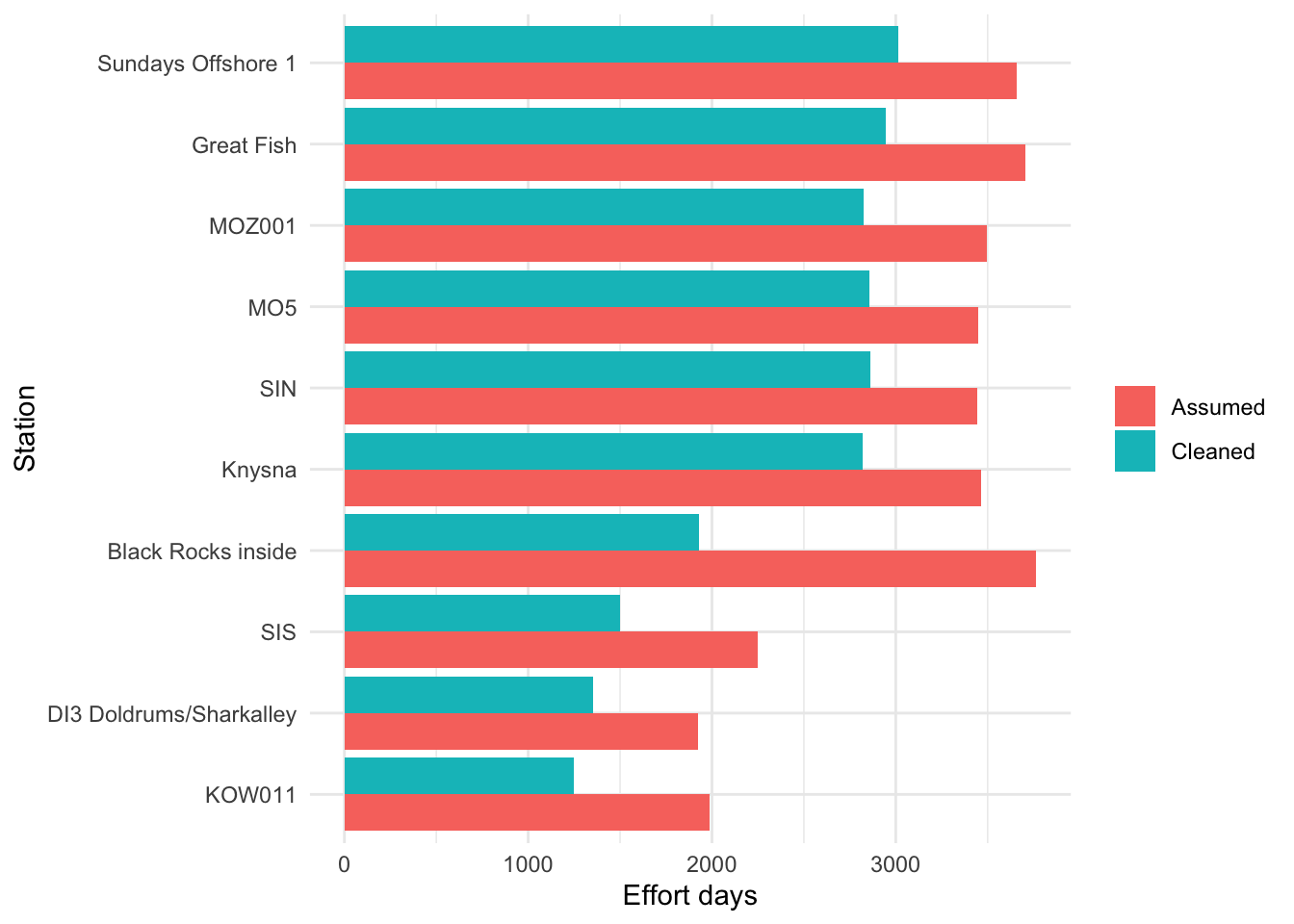

It might seem like a lot of effort to work this out for a 5% overestimate of time, but if you’re relying on some of these receivers as an indicator of core habitat then you’re going to get pretty significant zero-inflation as a result and bias your results. Therefore taking the time to really understand you foundational datasets gives you a better chance to defend your downstream analysis and you now know the array a little bit better.

Count unique receiver stations

How many unique receiver stations have been deployed in the ATAP network over time? Remember that you can’t rely on the obs in your environment to tell you how many stations were deployed, you know need to use distinct() since station name could appear on several rows.

Code

receiver_effort %>% 
  distinct(station_name) %>% 
  count()

# A tibble: 1 × 1
      n
  <int>
1   438

Add station coordinates back to the effort table.

Code

receiver_coords <- receiver %>% 
  dplyr::select(station_name, latitude, longitude) %>% 
  distinct()

receiver_effort <- receiver_effort %>% 
  left_join(receiver_coords, by = "station_name")

Export the cleaned receiver effort file.

Code

write.csv(
  receiver_effort,
  "data/receiver_effort_clean.csv",
  row.names = FALSE
)

Release locations

Release data can be built into the biometrics table, but some packages and workflows use a separate release-location file.

Code

release <- read_csv("data/tag_locations.csv")

release <- janitor::clean_names(release)

release <- release %>% 
  rename(
    latitude = lat,
    longitude = lon
  )

release

# A tibble: 7 × 3
  location latitude longitude
  <chr>       <dbl>     <dbl>
1 GB          -34.7      19.4
2 FB          -34.2      18.6
3 MB          -34.2      22.2
4 WLD         -34.0      22.6
5 PB          -34.1      23.4
6 JB          -34.1      25.0
7 PSJ         -31.7      29.6

Export the cleaned release file if needed.

Code

write.csv(
  release,
  "data/release_clean.csv",
  row.names = FALSE
)

Wrap-up

In this section we cleaned and checked the three core telemetry metadata tables:

biometrics
detections
receiver metadata
release sites

The most important lesson is that telemetry quality control is not just about making the data neat. It directly affects downstream estimates of detections, residency, movement, receiver effort, and bias. We’ve done all this without having to open Excel and manually wrangle data. This saves trying to figure out and remember what you clicked, changed or moved, so that you can execute scripts quickly and dig into the interesting stuff.